Skeleton Animation & Visualization

Posted Mar 28, 2025 Updated Mar 30, 2025

By Charles Cai 4 min read

Skeleton Animation & Visualization

“Get Animated, Stay Inspired”

Yushi Cai
March 2025

A Blog Series on Computer Graphics and Physical Simulation, aiming to provide insights into the implementation of various techniques and algorithms in the field. This series will cover topics such as mesh visualization, skeleton visualization, posed mesh visualization, and skeletal animation.

Overview

[Req.1 & 5] Mesh Visualization
[Req.2] Skeleton Visualization
[Req.3] Posed Mesh Visualization
[Req.4] Skeletal Animation
Pipeline Integration
References

Req.1 & 5 Mesh Visualization

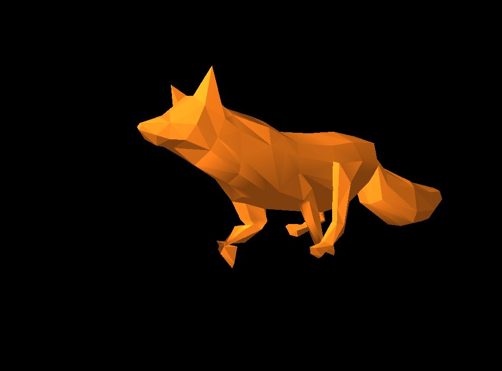
Implemented a real-time renderer with lighting to visualize the mesh. Using Blinn-Phong shading model, the mesh is rendered with a light source and a camera. The mesh is displayed in a GL_FILL mode to show the mesh structure.

Blinn-Phong shading is a method that calculates the color of a pixel based on the ambient, diffuse, and specular components of the light. The ambient component is the base color of the object, the diffuse component is the color of the object when lit by a light source, and the specular component is the color of the object when reflecting light. The Blinn-Phong model combines these components to create a realistic lighting effect.

Related files:

Implementation of Blin-Phong shading model

src/render/mesh/mesh.cpp
src/render/mesh/mesh.frag.inl
src/render/mesh/mesh.vert.inl

Enable GL_DEPTH_TEST to avoid ‘see-through’ effect

src/render/viewer/skinning_viewer.cpp

Core pseudo code:

  
// Blinn-Phong shading model
vec3 blinnPhong(vec3 normal, vec3 lightDir, vec3 viewDir, vec3 lightColor, vec3 objectColor) {
    // Ambient
    vec3 ambient = ambient_strength * objectColor;

    // Diffuse
    float diff = max(dot(normal, lightDir), 0.0);
    vec3 diffuse = diff * lightColor * objectColor;

    // Specular
    vec3 halfwayDir = normalize(lightDir + viewDir);
    float spec = pow(max(dot(normal, halfwayDir), 0.0), shininess);
    vec3 specular = spec * lightColor;

    return ambient + diffuse + specular;
}

Output:

Req.2 & 3 Skeleton Visualization & Posed Mesh Visualization

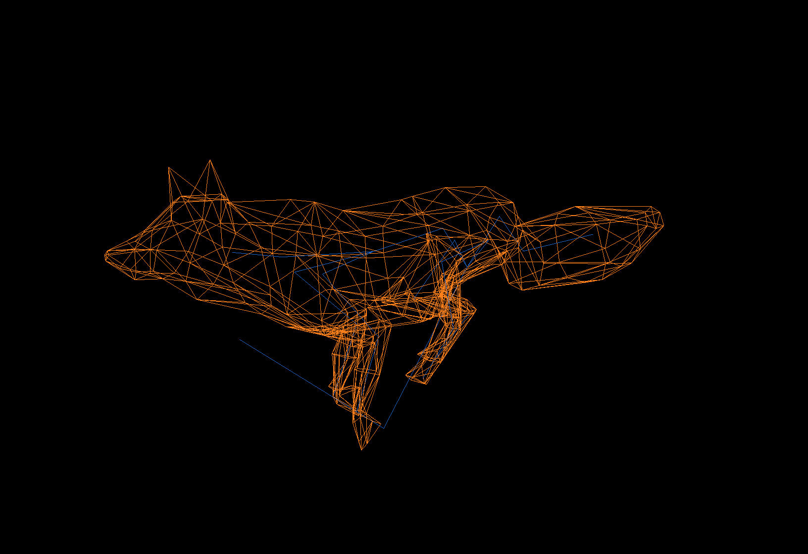
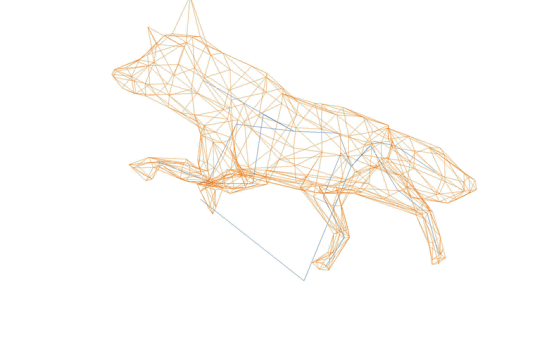
A hierarchy of bones is displayed using line segments for the poses. The skeleton is visualized with distinct colors for clarity. The skeleton is displayed in a GL_LINE mode to show the bone structure.

Related files:

Implementation of skeleton visualization

src/skeletal/skeleton.hpp
src/skeletal/skeleton.frag.inl (to change color)

Implementation of posed mesh visualization

src/viewer/skinned_viewer.cpp
src/mesh/mesh.vert.inl

Enable or disable skeleton visual display with flag RENDER_SKELETON

src/render/viewer/skinning_viewer.cpp

The CalcLocalTransformToParent() function is used to calculate the local transformation matrix for each bone in the skeleton, compared to its parent bone. Therefore, we perform a recursive traversal of the skeleton hierarchy to calculate the transformation matrix for each bone until we reach the root bone in CalcWorldTransform(). After that, we use CalcWorldPosition() to calculate the world position of each bone via translation Extraction ( so the matrix’s last column represents the translation component. Multiplying by (0,0,0,1) essentially “picks out” this translation component, refer to https://learnopengl.com/Getting-started/Transformations ).

Linear Blend Skinning (LBS)

The standard formulation of Linear Blend Skinning (LBS) is typically written as:

\[\mathbf{v}' = \sum_{i=1}^{n} w_i \left( \mathbf{T}_i \mathbf{B}_i^{-1} \right) \mathbf{v}\]

Where:

$ \mathbf{v} $ is the original vertex position in the rest (bind) pose.
$\mathbf{v}’$ is the deformed (skinned) vertex position.
$w_i$ is the weight associated with the $i$-th bone (with $\sum_i w_i = 1$).
$\mathbf{T}_i$ is the current transformation matrix (obtained from animation, such as through keyframe interpolation) for the $i$-th bone.
$\mathbf{B}_i^{-1}$ is the inverse of the bone’s bind pose (rest pose) matrix, which transforms the vertex from the bone’s local bind space back to the model space.

This is exactly what we implemented in skinned_viewer.cpp : $T_{joint} = \mathbf{T}_i \mathbf{B}_i^{-1}$. And then in mesh.vert.inl, we calculate the $\mathbf{v}’ = \sum_{i=1}^{n} w_i T_{joint} \mathbf{v}$ .

Output: Skeleton-Blue Mesh wirefram-Orange

skvis1 — Figure 2: Skeleton Black Vis with Skeleton:Blue & Mesh wirefram:Orange

skvis2 — Figure 3: Skeleton White Vis with Skeleton:Blue & Mesh wirefram:Orange

Req.4 & Pipeline Skeleton Animation

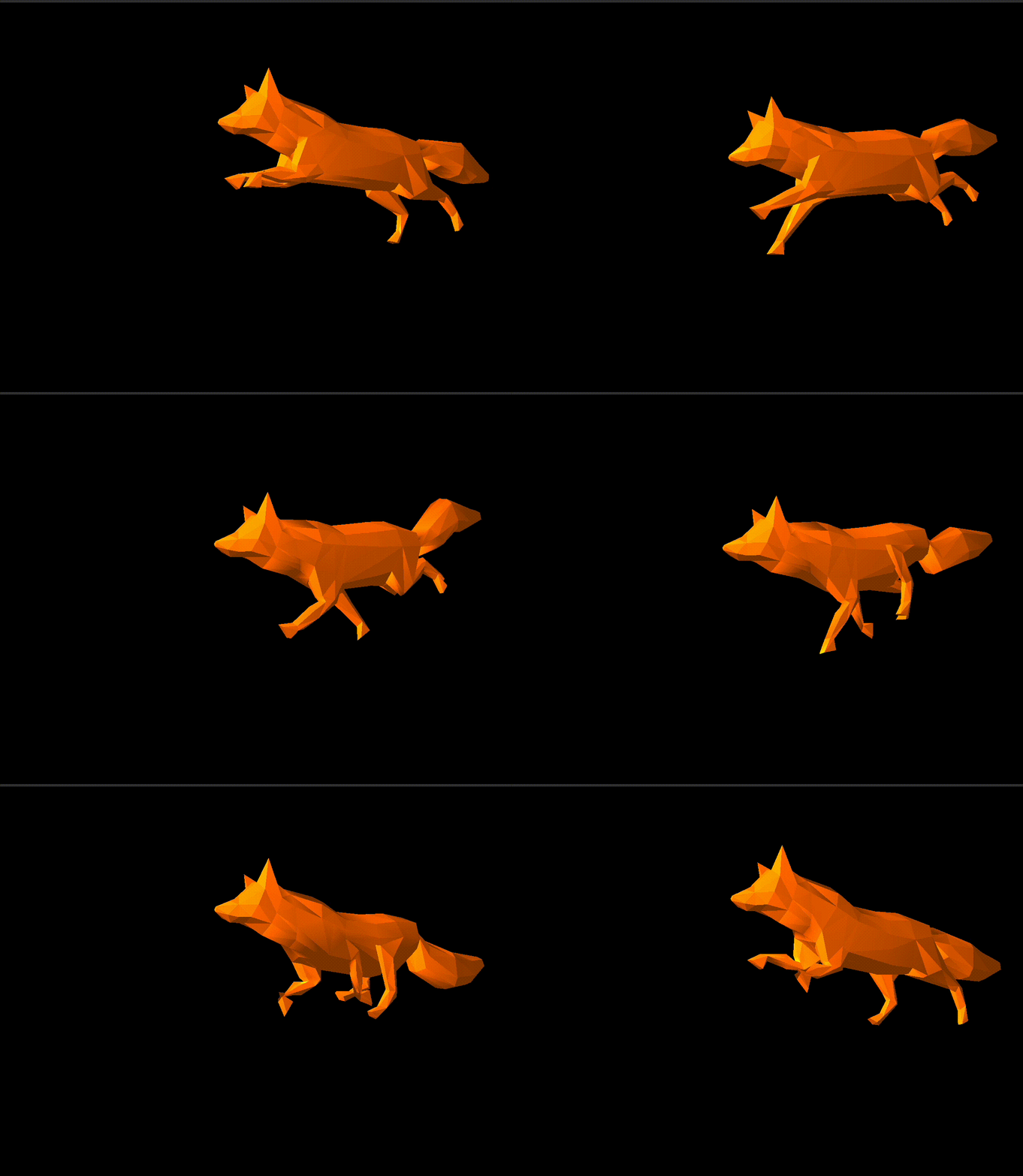
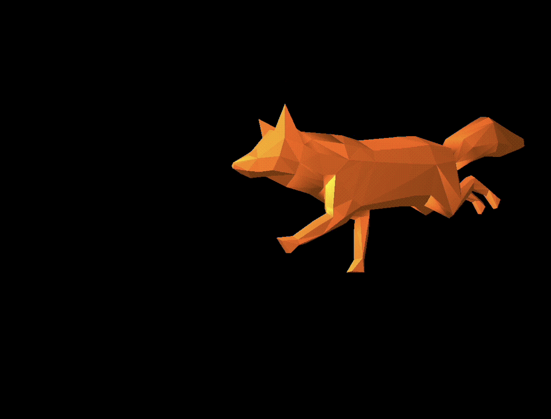
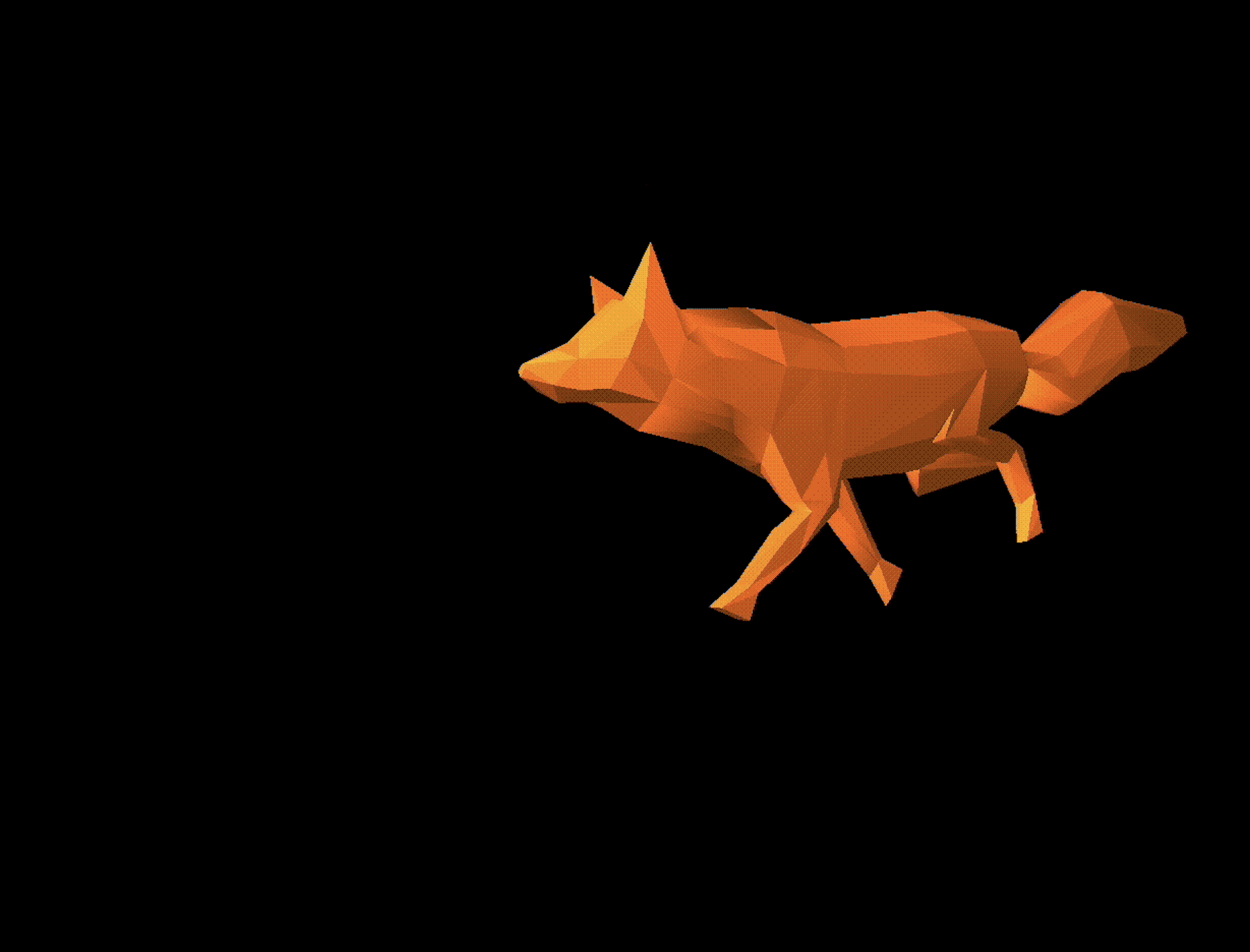
The animation is implemented using a keyframe-based approach. The skeleton is animated by interpolating between keyframes. The animation is displayed in real-time with a smooth transition between keyframes.

Related files:

Implementation of skeleton animation

src/skeletal/animation.hpp

First we have to locate the first element in the sorted key_time_data that is greater than time. This identifies the key frame immediately after the current time. Then we divided into 2 cases:

Case 1: Time is Between Two Key Frames so the key frame is not the first key frame, we need to interpolate between the two key frames. We calculate the interpolation factor alpha based on the time difference between the two key frames and the current time. The interpolation factor is then used to blend between the two key frames.
Case 2: Time is Before the First Key Frame: we simply return the first key frame.